McqMate
125
95.3k
180+ Control System Engineering (CSE) Solved MCQs
These multiple-choice questions (MCQs) are designed to enhance your knowledge and understanding in the following areas: Electrical Engineering .
| 51. |
For non-unity feedback system, the error is calculated with respect to the reference signal. |
| A. | true |
| B. | false |
| Answer» B. false | |
| Explanation: the error will be calculated with respect to the actuating signal i.e the feedback signal is either added or subtracted from the reference signal and the error is calculated with respect to the resultant signal. hence, the above statement is false. | |
| 52. |
Which of the following command will reveal the damping ratio of the system? |
| A. | damp() |
| B. | damp[] |
| C. | damping{} |
| D. | dr() |
| Answer» A. damp() | |
| Explanation: damp() is the correct command to find the damping ration of the system. we need to represent the system by it’s transfer function and give it as an input to the damp() | |
| 53. |
If the damping factor is zero, the unit-step response is |
| A. | purely sinusoidal |
| B. | ramp function |
| C. | pulse function |
| D. | impulse function |
| Answer» A. purely sinusoidal | |
| Explanation: the generalized time response of a second order control system reduces to a | |
| 54. |
If the damping ratio is equal to 1, a second-order system is |
| A. | having maginary roots of the characteristic equation |
| B. | underdamped |
| C. | critically damped with unequal roots |
| D. | critically damped with equal roots |
| Answer» D. critically damped with equal roots | |
| Explanation: the time response of a system with a damping ratio of 1 is critically damped. but the roots of the characteristic equation will be equal and equal to negative of the natural undamped frequency of the system. | |
| 55. |
From the following graphs of the generalized transfer function 1/s+a, which plot shows a transfer function with a bigger value of a? |
| A. | blue plot |
| B. | red plot |
| C. | yellow plot |
| D. | purple plot |
| Answer» D. purple plot | |
| Explanation: as the value of a increases, the inverse laplace transform of the given transfer function suggests that the e-at value is reducing. hence for a higher a, the graph reaches a 0 earlier. from the given figure, the purple plot reaches the steady state faster so purple plot is correct only. | |
| 56. |
From the following graphs of the generalized transfer function 1/as2, which plot shows the transfer function for a higher a? |
| A. | blue |
| B. | red |
| C. | yellow |
| D. | purple |
| Answer» D. purple | |
| Explanation: the impulse response of the given transfer function is a ramp function of slope 1/a. if a increases, the slope decreases. hence, from the above figure, purple is the correct one. | |
| 57. |
If the damping factor is less than the damping factor at critical damping, the time response of the system is |
| A. | underdamped |
| B. | overdamped |
| C. | marginally damped |
| D. | unstable |
| Answer» A. underdamped | |
| Explanation: if the damping factor is less than the damping factor at critical damping | |
| 58. |
This makes the system underdamped since the response of the system becomes a decaying sinusoid in nature. |
| A. | 9/(s2+2s+9) |
| B. | 16/(s2+2s+16) |
| C. | 25/(s2+2s+25) |
| D. | 36/(s2+2s+36) |
| Answer» D. 36/(s2+2s+36) | |
| Explanation: comparing the characteristic equation with the standard equation the value of the damping factor is calculated and the value for the option d is minimum hence the system will have the maximum overshoot . | |
| 59. |
The system in originally critically damped if the gain is doubled the system will be : |
| A. | remains same |
| B. | overdamped |
| C. | under damped |
| D. | undamped |
| Answer» C. under damped | |
| Explanation: hence due to this g lies between 0 and 1. | |
| 60. |
Let c(t) be the unit step response of a system with transfer function K(s+a)/(s+K). If c(0+) = 2 and c(∞) = 10, then the values of a and K are respectively. |
| A. | 2 and 10 |
| B. | -2 and 10 |
| C. | 10 and 2 |
| D. | 2 and -10 |
| Answer» C. 10 and 2 | |
| Explanation: applying initial value theorem which state that the initial value of the system is at time t =0 and this is used to find the value of k and final value theorem to find the value of a. | |
| 61. |
The damping ratio and peak overshoot are measures of: |
| A. | relative stability |
| B. | speed of response |
| C. | steady state error |
| D. | absolute stability |
| Answer» B. speed of response | |
| Explanation: speed of response is the speed at which the response takes the final value and this is determined by damping factor which reduces the oscillations and peak overshoot as the peak is less then the speed of response will be more. | |
| 62. |
A system has a complex conjugate root pair of multiplicity two or more in its characteristic equation. The impulse response of the system will be: |
| A. | a sinusoidal oscillation which decays exponentially; the system is therefore stable |
| B. | a sinusoidal oscillation with a time multiplier ; the system is therefore unstable |
| C. | a sinusoidal oscillation which rises exponentially ; the system is therefore unstable |
| D. | a dc term harmonic oscillation the system therefore becomes limiting stable |
| Answer» C. a sinusoidal oscillation which rises exponentially ; the system is therefore unstable | |
| Explanation: poles are the roots of the denominator of the transfer function and on imaginary axis makes the system stable but multiple poles makes the system unstable. | |
| 63. |
The step response of the system is c(t) = 10+8e-t-4/8e-2t . The gain in time constant form of transfer function will be: |
| A. | -7 |
| B. | 7 |
| C. | 7.5 |
| D. | -7.5 |
| Answer» D. -7.5 | |
| Explanation: differentiating the equation and getting the impulse response and then taking the inverse laplace transform and converting the form into time constant form we get k = | |
| 64. |
The steady state error for a unity feedback system for the input r(t) = Rt^2/2 to the system G(s) = K(s+2)/s(s3+7s2+12s) is |
| A. | 0 |
| B. | 6r/k |
| C. | ∞ |
| D. | 3r/k |
| Answer» B. 6r/k | |
| Explanation: ka = 2k/12 = k/6 | |
| 65. |
Find the velocity error constant of the system given below :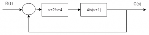
|
| A. | 0 |
| B. | 2 |
| C. | 4 |
| D. | ∞ |
| Answer» C. 4 | |
| Explanation: comparing with the characteristic equation the values of g and w are calculated as g = 1 and w = 4 and hence the system is critically damped. | |
| 66. |
Consider the unity feedback system with open loop transfer function the minimum value of the steady state error to a ramp input r(t) = 6tu(t) is OLTF = K/s(s+1)(s+2) |
| A. | 1 |
| B. | 2 |
| C. | 3 |
| D. | 4 |
| Answer» B. 2 | |
| Explanation: routh-hurwitz criterion is used to calculate the stability of the system by checking the sign changes of the first row and | |
| 67. |
A ramp input applied to a unity feedback system results in 5% steady state error. The type number and zero frequency gain of the system are respectively |
| A. | 1 and 20 |
| B. | 0 and 20 |
| C. | 0 and 1/20 |
| D. | 1 and 1/20 |
| Answer» A. 1 and 20 | |
| Explanation: steady state error is the error calculated between the final output and desired output and for the good control system the error must be less and this steady state error is inversely proportional to gain. | |
| 68. |
A particular control system yielded a steady state error of 0.20 for unit step input. A unit integrator is cascaded to this system and unit ramp input is applied to this modified system. What is the value of steady- state error for this modified system? |
| A. | 0.10 |
| B. | 0.15 |
| C. | 0.20 |
| D. | 0.25 |
| Answer» D. 0.25 | |
| Explanation: the integrator is similar to the phase lag systems and it is used to reduce or eleminate the steady state error and when it is cascaded with the ramp input hence the acceleration error constant is calculated which is equal to 0.25. | |
| 69. |
The error constants described are the ability to reduce the steady state errors. |
| A. | true |
| B. | false |
| Answer» A. true | |
| Explanation: as the type of the system becomes higher more steady state errors are eliminated. | |
| 70. |
Systems of type higher than 2 are not employed in practice. |
| A. | true |
| B. | false |
| Answer» A. true | |
| Explanation: these are more difficult to stabilize and dynamic errors are much larger. | |
| 71. |
Steady state refers to |
| A. | error at the steady state |
| B. | error at the transient state |
| C. | error at both state |
| D. | precision |
| Answer» A. error at the steady state | |
| Explanation: steady state errors are the change in the output at the steady state with respect to the change in the input. | |
| 72. |
The disadvantages of the error constants are: |
| A. | they do not give the information of the steady state error when the inputs are other than the three basic types |
| B. | error constant fail to indicate the exact manner in which the error function change with time. |
| C. | they do not give information of the steady state error and fail to indicate the exact manner in which the error function change with time |
| D. | they give information of the steady state error |
| Answer» C. they do not give information of the steady state error and fail to indicate the exact manner in which the error function change with time | |
| Explanation: the disadvantages of the error constants are as they do not give the information of the steady state error when the inputs are other than the three basic types and error constant fail to indicate the exact manner in which the error function change with time. | |
| 73. |
The input of a controller is |
| A. | sensed signal |
| B. | error signal |
| C. | desired variable value |
| D. | signal of fixed amplitude not dependent on desired variable value |
| Answer» B. error signal | |
| Explanation: controller is the block in the control system that control the input and provides the output and this is the first block of the system having the input as the error signal. | |
| 74. |
Phase lag controller: |
| A. | improvement in transient response |
| B. | reduction in steady state error |
| C. | reduction is settling time |
| D. | increase in damping constant |
| Answer» B. reduction in steady state error | |
| Explanation: phase lag controller is the integral controller that creates the phase lag and does not affect the value of the damping factor and that tries to reduce the steady state error. | |
| 75. |
Addition of zero at origin: |
| A. | improvement in transient response |
| B. | reduction in steady state error |
| C. | reduction is settling time |
| D. | increase in damping constant |
| Answer» A. improvement in transient response | |
| Explanation: stability of the system can be determined by various factors and for a good control system the stability of the system must be more and this can be increased by adding zero to the system and improves the transient response. | |
| 76. |
Derivative output compensation: |
| A. | improvement in transient response |
| B. | reduction in steady state error |
| C. | reduction is settling time |
| D. | increase in damping constant |
| Answer» C. reduction is settling time | |
| Explanation: derivative controller is the controller that is also like high pass filter and is also phase lead controller and it is used to increase the speed of response of the system by increasing the damping coefficient. | |
| 77. |
Derivative error compensation: |
| A. | improvement in transient response |
| B. | reduction in steady state error |
| C. | reduction is settling time |
| D. | increase in damping constant |
| Answer» D. increase in damping constant | |
| Explanation: damping constant reduces the gain, as it is inversely proportional to the gain and as increasing the damping gain reduces and hence the speed of response and bandwidth are both increased. | |
| 78. |
Lag compensation leads to: |
| A. | increases bandwidth |
| B. | attenuation |
| C. | increases damping factor |
| D. | second order |
| Answer» B. attenuation | |
| Explanation: phase compensation can be lead, lag or lead lag compensation and integral compensation is also known as lag compensation and leads to attenuation which has least effect on the speed but the accuracy is increased. | |
| 79. |
Lead compensation leads to: |
| A. | increases bandwidth |
| B. | attenuation |
| C. | increases damping factor |
| D. | second order |
| Answer» A. increases bandwidth | |
| Explanation: high pass filter is similar to the phase lead compensation and leads to increase in bandwidth and also increase in speed of response. | |
| 80. |
Lag-lead compensation is a: |
| A. | increases bandwidth |
| B. | attenuation |
| C. | increases damping factor |
| D. | second order |
| Answer» D. second order | |
| Explanation: lag-lead compensation is a second order control system which has lead and lag compensation both and thus has combined effect of both lead and lag compensation this is obtained by the differential equation. | |
| 81. |
Rate compensation : |
| A. | increases bandwidth |
| B. | attenuation |
| C. | increases damping factor |
| D. | second order |
| Answer» C. increases damping factor | |
| Explanation: damping factor is increased for reducing the oscillations and increasing the stability and speed of response which are the essential requirements of the control system and damping factor is increased by the rate compensation. | |
| 82. |
Negative exponential term in the equation of the transfer function causes the transportation lag. |
| A. | true |
| B. | false |
| Answer» A. true | |
| Explanation: transportation lag is the lag that is generally neglected in systems but for the accurate measurements the delay caused to transport the input from one end to the other is called the transportation lag in the system causes instability to the system. | |
| 83. |
Scientist Bode have contribution in : |
| A. | asymptotic plots |
| B. | polar plots |
| C. | root locus technique |
| D. | constant m and n circle |
| Answer» A. asymptotic plots | |
| Explanation: asymptotic plots are the bode plots that are drawn to find the relative stability of the system by finding the phase and gain margin and this was invented by scientist bode. | |
| 84. |
Scientist Evans have contribution in : |
| A. | asymptotic plots |
| B. | polar plots |
| C. | root locus technique |
| D. | constant m and n circle |
| Answer» C. root locus technique | |
| Explanation: root locus technique is used to find the transient and steady state response characteristics by finding the locus of the gain of the system and this was made scientist evans . | |
| 85. |
Scientist Nyquist have contribution in: |
| A. | asymptotic plots |
| B. | polar plots |
| C. | root locus technique |
| D. | constant m and n circle |
| Answer» B. polar plots | |
| Explanation: nyquist plot is used to find the stability of the system by open loop poles and zeroes and the encirclements of the poles and zeroes and satisfying the equation n=p-z and this is named under the name of scientist nyquist. | |
| 86. |
Which one of the following methods can determine the closed loop system resonance frequency operation? |
| A. | root locus method |
| B. | nyquist method |
| C. | bode plot |
| D. | m and n circle |
| Answer» D. m and n circle | |
| Explanation: closed loop system resonance frequency is the frequency at which maximum peak occurs and this frequency of operation can best be determined with the help of m and n circle. | |
| 87. |
If the gain of the open loop system is doubled, the gain of the system is : |
| A. | not affected |
| B. | doubled |
| C. | halved |
| D. | one fourth of the original value |
| Answer» A. not affected | |
| Explanation: gain of the open loop system is doubled then the gain of the system is not affected as the gain of the system is not dependent on the overall gain of the system. | |
| 88. |
Constant M- loci: |
| A. | constant gain and constant phase shift loci of the closed-loop system. |
| B. | plot of loop gain with the variation in frequency |
| C. | circles of constant gain for the closed loop transfer function |
| D. | circles of constant phase shift for the closed loop transfer function |
| Answer» D. circles of constant phase shift for the closed loop transfer function | |
| Explanation: by definition, constant m loci are circles of constant phase shift for the closed loop transfer function. | |
| 89. |
Constant N-loci: |
| A. | constant gain and constant phase shift loci of the closed-loop system. |
| B. | plot of loop gain with the variation in frequency |
| C. | circles of constant gain for the closed loop transfer function |
| D. | circles of constant phase shift for the closed loop transfer function |
| Answer» C. circles of constant gain for the closed loop transfer function | |
| Explanation: constant n loci are the circles of constant gain for the closed loop transfer function and the intersection point of the m and n is always the point (-1,0). | |
| 90. |
Nichol’s chart: |
| A. | constant gain and constant phase shift loci of the closed-loop system. |
| B. | plot of loop gain with the variation in frequency |
| C. | circles of constant gain for the closed loop transfer function |
| D. | circles of constant phase shift for the closed loop transfer function |
| Answer» B. plot of loop gain with the variation in frequency | |
| Explanation: nichol’s chart are plot of loop gain with the variation in frequency and this is used to determine the stability of the system with the variation in the frequency. | |
| 91. |
For a stable closed loop system, the gain at phase crossover frequency should always be: |
| A. | < 20 db |
| B. | < 6 db |
| C. | > 6 db |
| D. | > 0 db |
| Answer» D. > 0 db | |
| Explanation: phase crossover frequency is the frequency at which the gain of the system must be 1 and for a stable system the gain is decibels must be 0 db. | |
| 92. |
Which principle specifies the relationship between enclosure of poles & zeros by s- plane contour and the encirclement of origin by q(s) plane contour? |
| A. | argument |
| B. | agreement |
| C. | assessment |
| D. | assortment |
| Answer» A. argument | |
| Explanation: argument principle specifies the relationship between enclosure of poles & zeros by s-plane contour and the encirclement of origin by q(s) plane contour. | |
| 93. |
If a Nyquist plot of G (jω) H (jω) for a closed loop system passes through (-2, j0) point in GH plane, what would be the value of gain margin of the system in dB? |
| A. | 0 db |
| B. | 2.0201 db |
| C. | 4 db |
| D. | 6.0205 db |
| Answer» D. 6.0205 db | |
| Explanation: gain margin is calculated by taking inverse of the gain where the nyquist plot cuts the real axis. | |
| 94. |
For Nyquist contour, the size of radius is |
| A. | 25 |
| B. | 0 |
| C. | 1 |
| D. | ∞ |
| Answer» D. ∞ | |
| Explanation: for nyquist contour, the size of radius is ∞. | |
| 95. |
According to Nyquist stability criterion, where should be the position of all zeros of q(s) corresponding to s-plane? |
| A. | on left half |
| B. | at the center |
| C. | on right half |
| D. | random |
| Answer» A. on left half | |
| Explanation: according to nyquist stability criterion zeroes must lie on the left half on the s plane. | |
| 96. |
If the system is represented by G(s) H(s) = k (s+7) / s (s +3) (s + 2), what would be its magnitude at ω = ∞? |
| A. | 0 |
| B. | ∞ |
| C. | 7/10 |
| D. | 21 |
| Answer» A. 0 | |
| Explanation: on calculating the magnitude | |
| 97. |
Consider the system represented by the equation given below. What would be the total phase value at ω = 0? |
| A. | -90° |
| B. | -180° |
| C. | -270° |
| D. | -360° |
| Answer» C. -270° | |
| Explanation: the phase can be calculated by the basic formula for calculating phase angle. | |
| 98. |
In polar plots, if a pole is added at the origin, what would be the value of the magnitude at Ω = 0? |
| A. | zero |
| B. | infinity |
| C. | unity |
| D. | unpredictable |
| Answer» B. infinity | |
| Explanation: addition of pole causes instability to the system. | |
| 99. |
In polar plots, what does each and every point represent w.r.t magnitude and angle? |
| A. | scalar |
| B. | vector |
| C. | phasor |
| D. | differentiator |
| Answer» C. phasor | |
| Explanation: each and every point on the | |
| 100. |
A system has poles at 0.01 Hz, 1 Hz and 80Hz, zeroes at 5Hz, 100Hz and 200Hz. The approximate phase of the system response at 20 Hz is : |
| A. | -90° |
| B. | 0° |
| C. | 90° |
| D. | -180° |
| Answer» A. -90° | |
| Explanation: pole at 0.01 hz gives -180° phase. zero at 5hz gives 90° phase therefore at 20hz -90° phase shift is provided. | |
Done Studing? Take A Test.
Great job completing your study session! Now it's time to put your knowledge to the test. Challenge yourself, see how much you've learned, and identify areas for improvement. Don’t worry, this is all part of the journey to mastery. Ready for the next step? Take a quiz to solidify what you've just studied.